我的书签
我的书签
 添加书签
添加书签 移除书签
移除书签- 二十、将子图应用于我们的图表
二十、将子图应用于我们的图表
在这个 Matplotlib 教程中,我们将处理我们以前教程的代码,并实现上一个教程中的子图配置。 我们的起始代码是这样:
import matplotlib.pyplot as pltimport matplotlib.dates as mdatesimport matplotlib.ticker as mtickerfrom matplotlib.finance import candlestick_ohlcfrom matplotlib import styleimport numpy as npimport urllibimport datetime as dtstyle.use('fivethirtyeight')print(plt.style.available)print(plt.__file__)def bytespdate2num(fmt, encoding='utf-8'):strconverter = mdates.strpdate2num(fmt)def bytesconverter(b):s = b.decode(encoding)return strconverter(s)return bytesconverterdef graph_data(stock):fig = plt.figure()ax1 = plt.subplot2grid((1,1), (0,0))stock_price_url = 'http://chartapi.finance.yahoo.com/instrument/1.0/'+stock+'/chartdata;type=quote;range=1m/csv'source_code = urllib.request.urlopen(stock_price_url).read().decode()stock_data = []split_source = source_code.split('\n')for line in split_source:split_line = line.split(',')if len(split_line) == 6:if 'values' not in line and 'labels' not in line:stock_data.append(line)date, closep, highp, lowp, openp, volume = np.loadtxt(stock_data,delimiter=',',unpack=True,converters={0: bytespdate2num('%Y%m%d')})x = 0y = len(date)ohlc = []while x < y:append_me = date[x], openp[x], highp[x], lowp[x], closep[x], volume[x]ohlc.append(append_me)x+=1candlestick_ohlc(ax1, ohlc, width=0.4, colorup='#77d879', colordown='#db3f3f')for label in ax1.xaxis.get_ticklabels():label.set_rotation(45)ax1.xaxis.set_major_formatter(mdates.DateFormatter('%Y-%m-%d'))ax1.xaxis.set_major_locator(mticker.MaxNLocator(10))ax1.grid(True)bbox_props = dict(boxstyle='round',fc='w', ec='k',lw=1)ax1.annotate(str(closep[-1]), (date[-1], closep[-1]),xytext = (date[-1]+4, closep[-1]), bbox=bbox_props)## # Annotation example with arrow## ax1.annotate('Bad News!',(date[11],highp[11]),## xytext=(0.8, 0.9), textcoords='axes fraction',## arrowprops = dict(facecolor='grey',color='grey'))###### # Font dict example## font_dict = {'family':'serif',## 'color':'darkred',## 'size':15}## # Hard coded text## ax1.text(date[10], closep[1],'Text Example', fontdict=font_dict)plt.xlabel('Date')plt.ylabel('Price')plt.title(stock)#plt.legend()plt.subplots_adjust(left=0.11, bottom=0.24, right=0.90, top=0.90, wspace=0.2, hspace=0)plt.show()graph_data('EBAY')
一个主要的改动是修改轴域的定义:
ax1 = plt.subplot2grid((6,1), (0,0), rowspan=1, colspan=1)plt.title(stock)ax2 = plt.subplot2grid((6,1), (1,0), rowspan=4, colspan=1)plt.xlabel('Date')plt.ylabel('Price')ax3 = plt.subplot2grid((6,1), (5,0), rowspan=1, colspan=1)
现在,ax2是我们实际上在绘制的股票价格数据。 顶部和底部图表将作为指标信息。
在我们绘制数据的代码中,我们需要将ax1更改为ax2:
candlestick_ohlc(ax2, ohlc, width=0.4, colorup='#77d879', colordown='#db3f3f')for label in ax2.xaxis.get_ticklabels():label.set_rotation(45)ax2.xaxis.set_major_formatter(mdates.DateFormatter('%Y-%m-%d'))ax2.xaxis.set_major_locator(mticker.MaxNLocator(10))ax2.grid(True)bbox_props = dict(boxstyle='round',fc='w', ec='k',lw=1)ax2.annotate(str(closep[-1]), (date[-1], closep[-1]),xytext = (date[-1]+4, closep[-1]), bbox=bbox_props)
更改之后,代码为:
import matplotlib.pyplot as pltimport matplotlib.dates as mdatesimport matplotlib.ticker as mtickerfrom matplotlib.finance import candlestick_ohlcfrom matplotlib import styleimport numpy as npimport urllibimport datetime as dtstyle.use('fivethirtyeight')print(plt.style.available)print(plt.__file__)def bytespdate2num(fmt, encoding='utf-8'):strconverter = mdates.strpdate2num(fmt)def bytesconverter(b):s = b.decode(encoding)return strconverter(s)return bytesconverterdef graph_data(stock):fig = plt.figure()ax1 = plt.subplot2grid((6,1), (0,0), rowspan=1, colspan=1)plt.title(stock)ax2 = plt.subplot2grid((6,1), (1,0), rowspan=4, colspan=1)plt.xlabel('Date')plt.ylabel('Price')ax3 = plt.subplot2grid((6,1), (5,0), rowspan=1, colspan=1)stock_price_url = 'http://chartapi.finance.yahoo.com/instrument/1.0/'+stock+'/chartdata;type=quote;range=1m/csv'source_code = urllib.request.urlopen(stock_price_url).read().decode()stock_data = []split_source = source_code.split('\n')for line in split_source:split_line = line.split(',')if len(split_line) == 6:if 'values' not in line and 'labels' not in line:stock_data.append(line)date, closep, highp, lowp, openp, volume = np.loadtxt(stock_data,delimiter=',',unpack=True,converters={0: bytespdate2num('%Y%m%d')})x = 0y = len(date)ohlc = []while x < y:append_me = date[x], openp[x], highp[x], lowp[x], closep[x], volume[x]ohlc.append(append_me)x+=1candlestick_ohlc(ax2, ohlc, width=0.4, colorup='#77d879', colordown='#db3f3f')for label in ax2.xaxis.get_ticklabels():label.set_rotation(45)ax2.xaxis.set_major_formatter(mdates.DateFormatter('%Y-%m-%d'))ax2.xaxis.set_major_locator(mticker.MaxNLocator(10))ax2.grid(True)bbox_props = dict(boxstyle='round',fc='w', ec='k',lw=1)ax2.annotate(str(closep[-1]), (date[-1], closep[-1]),xytext = (date[-1]+4, closep[-1]), bbox=bbox_props)## # Annotation example with arrow## ax1.annotate('Bad News!',(date[11],highp[11]),## xytext=(0.8, 0.9), textcoords='axes fraction',## arrowprops = dict(facecolor='grey',color='grey'))###### # Font dict example## font_dict = {'family':'serif',## 'color':'darkred',## 'size':15}## # Hard coded text## ax1.text(date[10], closep[1],'Text Example', fontdict=font_dict)##plt.legend()plt.subplots_adjust(left=0.11, bottom=0.24, right=0.90, top=0.90, wspace=0.2, hspace=0)plt.show()graph_data('EBAY')
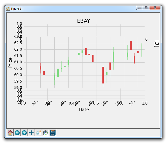
结果为: