 我的书签
我的书签
 添加书签
添加书签 移除书签
移除书签- 第十八课:Billbard和粒子
- 方案1:2D法
- 方案2:3D法
- 方案3:固定大小3D法
- 方案4:限制垂直旋转法
- 粒子(Particles)与实例(Instancing)
- 一大波粒子正在接近中……
- 实例
- 意义何在?
- 生与死
- 创建新粒子
- 删除旧粒子
- 仿真主循环
- 排序
- 延伸课题
- 动画粒子
- 处理多个粒子系统
- 平滑粒子
- 提高填充率
- 粒子物理效果
- GPU仿真
- 一大波粒子正在接近中……
第十八课:Billbard和粒子
公告板是3D世界中的2D元素。它既不是最顶层的2D菜单,也不是可以随意转动的3D平面,而是介于两者之间的一种元素,比如游戏中的血条。
公告板的独特之处在于:它位于某个特定位置,朝向是自动计算的,这样它就能始终面向相机(观察者)。
方案1:2D法
2D法十分简单。只需计算出点在屏幕空间的坐标,然后在该处显示2D文本(参见第十一课)即可。
// Everything here is explained in Tutorial 3 ! There's nothing new.glm::vec4 BillboardPos_worldspace(x,y,z, 1.0f);glm::vec4 BillboardPos_screenspace = ProjectionMatrix * ViewMatrix * BillboardPos_worldspace;BillboardPos_screenspace /= BillboardPos_screenspace.w;if (BillboardPos_screenspace.z < 0.0f){// Object is behind the camera, don't display it.}
就这么搞定了!
2D法优点是简单易行,无论点与相机距离远近,公告板始终保持大小不变。但此法总是把文本显示在最顶层,有可能会遮挡其他物体,影响渲染效果。
方案2:3D法
与2D法相比,3D法常常效果更好,也没复杂多少。
我们的目的就是无论相机如何移动,都要让公告板网格正对着相机:
可将此视为模型矩阵的构造问题之简化版。基本思路是将公告板的各角落置于 (存疑待查)The idea is that each corner of the billboard is at the center position, displaced by the camera’s up and right vectors :
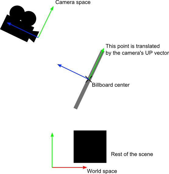
当然,我们仅仅知道世界空间中的公告板中心位置,因此还需要相机在世界空间中的up/right向量。
在相机空间,相机的up向量为(0,1,0)。要把up向量变换到世界空间,只需乘以观察矩阵的逆矩阵(由相机空间变换至世界空间的矩阵)。
用数学公式表示即:
CameraRight_worldspace = {ViewMatrix[0][0], ViewMatrix[1][0], ViewMatrix[2][0]}
CameraUp_worldspace = {ViewMatrix[0][1], ViewMatrix[1][1], ViewMatrix[2][1]}
接下来,顶点坐标的计算就很简单了:
vec3 vertexPosition_worldspace =particleCenter_wordspace+ CameraRight_worldspace * squareVertices.x * BillboardSize.x+ CameraUp_worldspace * squareVertices.y * BillboardSize.y;
particleCenter_worldspace顾名思义即公告板的中心位置,以vec3类型的uniform变量表示。squareVertices是原始的网格。左顶点的squareVertices.x为-0.5(存疑待查),which are thus moved towars the left of the camera (because of the *CameraRight_worldspace)BillboardSize是公告板大小,以世界单位为单位,uniform变量。
效果如下。怎么样,是不是很简单?
为了保证内容完整性,这里给出squareVertices的数据:
// The VBO containing the 4 vertices of the particles.static const GLfloat g_vertex_buffer_data[] = {-0.5f, -0.5f, 0.0f,0.5f, -0.5f, 0.0f,-0.5f, 0.5f, 0.0f,0.5f, 0.5f, 0.0f,};
方案3:固定大小3D法
正如上面所看到的,公告板大小随着相机与之的距离变化。有些情况下的确需要这样的效果,但血条这类公告板则需要保持大小不变。
vertexPosition_worldspace = particleCenter_wordspace;// Get the screen-space position of the particle's centergl_Position = VP * vec4(vertexPosition_worldspace, 1.0f);// Here we have to do the perspective division ourselves.gl_Position /= gl_Position.w;// Move the vertex in directly screen space. No need for CameraUp/Right_worlspace here.gl_Position.xy += squareVertices.xy * vec2(0.2, 0.05);
方案4:限制垂直旋转法
一些引擎以公告板表示远处的树和灯。不过,这些树可不能任意转向,必须是竖直的。So you need an hybrid system that rotates only around one axis.(存疑待查)
这个方案作为练习留给读者。
粒子(Particles)与实例(Instancing)
粒子与3D公告板很类似。不过,粒子有如下四个特点:
- 数量较大
- 可以运动
- 有生有死
- 半透明
伴随这些特点而来的是一系列问题。本课仅介绍其中一种解决方案,其他解决方案还多着呢……
一大波粒子正在接近中……
首先想到的思路就是套用上一课的代码,调用glDrawArrays逐个绘制粒子。这可不是个好办法。因为这种思路意味着你那锃光瓦亮的GTX 512显卡一次只能绘制一个四边形(很明显,性能损失高达99%)。就这么一个接一个地绘制公告板。
显然,我们得一次性绘制所有的粒子。
方法有很多种,如下是其中三种:
- 生成一个VBO,将所有粒子置于其中。简单,有效,在各种平台上均可行。
- 使用geometry shader。这不在本教程范围内,主要是因为50%的机器不支持该特性。
- 使用实例(instancing)。大部分机器都支持该特性。
本课将采用第三种方法。这种方法兼具性能优势和普适性,更重要的是,如果此法行得通,那第一种方法也就轻而易举了。
实例
“实例”的意思是以一个网格(比如本课中由两个三角形组成的四边形)为蓝本,创建多个该网格的实例。
具体地讲,我们通过如下一些buffer实现instancing:
- 一部分用于描述原始网格
- 一部分用于描述各实例的特性
这些buffer的内容可自行选择。在我们这个简单的例子包含了:
- 一个网格顶点buffer。没有index buffer,因此一共有6个
vec3变量,构成两个三角形,进而组合成一个四边形。 - 一个buffer存储粒子的中心。
- 一个buffer存储粒子的颜色。
这些buffer都是标准buffer。创建方式如下:
// The VBO containing the 4 vertices of the particles.// Thanks to instancing, they will be shared by all particles.static const GLfloat g_vertex_buffer_data[] = {-0.5f, -0.5f, 0.0f,0.5f, -0.5f, 0.0f,-0.5f, 0.5f, 0.0f,0.5f, 0.5f, 0.0f,};GLuint billboard_vertex_buffer;glGenBuffers(1, &billboard_vertex_buffer);glBindBuffer(GL_ARRAY_BUFFER, billboard_vertex_buffer);glBufferData(GL_ARRAY_BUFFER, sizeof(g_vertex_buffer_data), g_vertex_buffer_data, GL_STATIC_DRAW);// The VBO containing the positions and sizes of the particlesGLuint particles_position_buffer;glGenBuffers(1, &particles_position_buffer);glBindBuffer(GL_ARRAY_BUFFER, particles_position_buffer);// Initialize with empty (NULL) buffer : it will be updated later, each frame.glBufferData(GL_ARRAY_BUFFER, MaxParticles * 4 * sizeof(GLfloat), NULL, GL_STREAM_DRAW);// The VBO containing the colors of the particlesGLuint particles_color_buffer;glGenBuffers(1, &particles_color_buffer);glBindBuffer(GL_ARRAY_BUFFER, particles_color_buffer);// Initialize with empty (NULL) buffer : it will be updated later, each frame.glBufferData(GL_ARRAY_BUFFER, MaxParticles * 4 * sizeof(GLubyte), NULL, GL_STREAM_DRAW);
粒子更新方法如下:
// Update the buffers that OpenGL uses for rendering.// There are much more sophisticated means to stream data from the CPU to the GPU,// but this is outside the scope of this tutorial.// http://www.opengl.org/wiki/Buffer_Object_StreamingglBindBuffer(GL_ARRAY_BUFFER, particles_position_buffer);glBufferData(GL_ARRAY_BUFFER, MaxParticles * 4 * sizeof(GLfloat), NULL, GL_STREAM_DRAW); // Buffer orphaning, a common way to improve streaming perf. See above link for details.glBufferSubData(GL_ARRAY_BUFFER, 0, ParticlesCount * sizeof(GLfloat) * 4, g_particule_position_size_data);glBindBuffer(GL_ARRAY_BUFFER, particles_color_buffer);glBufferData(GL_ARRAY_BUFFER, MaxParticles * 4 * sizeof(GLubyte), NULL, GL_STREAM_DRAW); // Buffer orphaning, a common way to improve streaming perf. See above link for details.glBufferSubData(GL_ARRAY_BUFFER, 0, ParticlesCount * sizeof(GLubyte) * 4, g_particule_color_data);
绘制之前还需绑定buffer。绑定方法如下:
// 1rst attribute buffer : verticesglEnableVertexAttribArray(0);glBindBuffer(GL_ARRAY_BUFFER, billboard_vertex_buffer);glVertexAttribPointer(0, // attribute. No particular reason for 0, but must match the layout in the shader.3, // sizeGL_FLOAT, // typeGL_FALSE, // normalized?0, // stride(void*)0 // array buffer offset);// 2nd attribute buffer : positions of particles' centersglEnableVertexAttribArray(1);glBindBuffer(GL_ARRAY_BUFFER, particles_position_buffer);glVertexAttribPointer(1, // attribute. No particular reason for 1, but must match the layout in the shader.4, // size : x + y + z + size => 4GL_FLOAT, // typeGL_FALSE, // normalized?0, // stride(void*)0 // array buffer offset);// 3rd attribute buffer : particles' colorsglEnableVertexAttribArray(2);glBindBuffer(GL_ARRAY_BUFFER, particles_color_buffer);glVertexAttribPointer(2, // attribute. No particular reason for 1, but must match the layout in the shader.4, // size : r + g + b + a => 4GL_UNSIGNED_BYTE, // typeGL_TRUE, // normalized? *** YES, this means that the unsigned char[4] will be accessible with a vec4 (floats) in the shader ***0, // stride(void*)0 // array buffer offset);
绘制方法与以往有所不同。这次不使用glDrawArrays或者glDrawElements(如果原始网格有index buffer的话)。这次用的是glDrawArraysInstanced或者glDrawElementsInstanced,效果等同于调用glDrawArraysN次(N是最后一个参数,此例中即ParticlesCount)。
glDrawArraysInstanced(GL_TRIANGLE_STRIP, 0, 4, ParticlesCount);
有件事差点忘了。我们还没告诉OpenGL哪个buffer是原始网格,哪些buffer是各实例的特性。调用glVertexAttribDivisor即可完成。有完整注释的代码如下:
// These functions are specific to glDrawArrays*Instanced*.// The first parameter is the attribute buffer we're talking about.// The second parameter is the "rate at which generic vertex attributes advance when rendering multiple instances"// http://www.opengl.org/sdk/docs/man/xhtml/glVertexAttribDivisor.xmlglVertexAttribDivisor(0, 0); // particles vertices : always reuse the same 4 vertices -> 0glVertexAttribDivisor(1, 1); // positions : one per quad (its center) -> 1glVertexAttribDivisor(2, 1); // color : one per quad -> 1// Draw the particules !// This draws many times a small triangle_strip (which looks like a quad).// This is equivalent to :// for(i in ParticlesCount) : glDrawArrays(GL_TRIANGLE_STRIP, 0, 4),// but faster.glDrawArraysInstanced(GL_TRIANGLE_STRIP, 0, 4, ParticlesCount);
如你所见,instancing是很灵活的,你可以将AttribDivisor设为任意整数。例如,’glVertexAttribDivisor(2, 10)’即设置后续10个实例都拥有相同的颜色。
意义何在?
意义在于如今我们只需在每帧中更新一个很小的buffer(粒子中心位置),而非整个网格。如此一来,带宽利用效率提升了4倍。
生与死
于场景中其它对象不同的是,粒子的生死更替十分频繁。我们得用一种速度相当快的方式来创建新粒子,抛弃旧粒子。new Particle()这种办法显然不够好。
创建新粒子
首先得创建一个大的粒子容器:
// CPU representation of a particlestruct Particle{glm::vec3 pos, speed;unsigned char r,g,b,a; // Colorfloat size, angle, weight;float life; // Remaining life of the particle. if < 0 : dead and unused.};const int MaxParticles = 100000;Particle ParticlesContainer[MaxParticles];
接下来,我们得想办法创建新粒子。如下的函数在ParticleContainer中线性搜索(听起来有些暴力)新粒子。不过,它是从上次已知位置开始搜索的,因此一般很快就返回了。
int LastUsedParticle = 0;// Finds a Particle in ParticlesContainer which isn't used yet.// (i.e. life < 0);int FindUnusedParticle(){for(int i=LastUsedParticle; i<MaxParticles; i++){if (ParticlesContainer[i].life < 0){LastUsedParticle = i;return i;}}for(int i=0; i<LastUsedParticle; i++){if (ParticlesContainer[i].life < 0){LastUsedParticle = i;return i;}}return 0; // All particles are taken, override the first one}
现在我们可以把ParticlesContainer[particleIndex]当中的life、color、speed和position设置成一些有趣的值。欲知详情请看代码,此处大有文章可作。我们比较关心的是每一帧中要生成多少粒子。这跟具体的应用有关,我们就设为每秒10000个(噢噢,略多啊)新粒子好了:
int newparticles = (int)(deltaTime*10000.0);
记得把个数限定在一个固定范围内:
// Generate 10 new particule each millisecond,// but limit this to 16 ms (60 fps), or if you have 1 long frame (1sec),// newparticles will be huge and the next frame even longer.int newparticles = (int)(deltaTime*10000.0);if (newparticles > (int)(0.016f*10000.0))newparticles = (int)(0.016f*10000.0);
删除旧粒子
这个需要一些技巧,参见下文=)
仿真主循环
ParticlesContainer同时容纳了“活着的”和“死亡的”粒子,但发送到GPU的buffer仅含活着的粒子。
所以,我们要遍历每个粒子,看它是否是活着的,是否应该“处死”。如果一切正常,那就添加重力,最后将其拷贝到GPU上相应的buffer中。
// Simulate all particlesint ParticlesCount = 0;for(int i=0; i<MaxParticles; i++){Particle& p = ParticlesContainer[i]; // shortcutif(p.life > 0.0f){// Decrease lifep.life -= delta;if (p.life > 0.0f){// Simulate simple physics : gravity only, no collisionsp.speed += glm::vec3(0.0f,-9.81f, 0.0f) * (float)delta * 0.5f;p.pos += p.speed * (float)delta;p.cameradistance = glm::length2( p.pos - CameraPosition );//ParticlesContainer[i].pos += glm::vec3(0.0f,10.0f, 0.0f) * (float)delta;// Fill the GPU bufferg_particule_position_size_data[4*ParticlesCount+0] = p.pos.x;g_particule_position_size_data[4*ParticlesCount+1] = p.pos.y;g_particule_position_size_data[4*ParticlesCount+2] = p.pos.z;g_particule_position_size_data[4*ParticlesCount+3] = p.size;g_particule_color_data[4*ParticlesCount+0] = p.r;g_particule_color_data[4*ParticlesCount+1] = p.g;g_particule_color_data[4*ParticlesCount+2] = p.b;g_particule_color_data[4*ParticlesCount+3] = p.a;}else{// Particles that just died will be put at the end of the buffer in SortParticles();p.cameradistance = -1.0f;}ParticlesCount++;}}
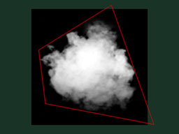
如下所示,效果看上去差不多了,不过还有一个问题……
排序
正如[第十课][1]中所讲,你必须按从后往前的顺序对半透明对象排序,方可获得正确的混合效果。
void SortParticles(){std::sort(&ParticlesContainer[0], &ParticlesContainer[MaxParticles]);}
std::sort需要一个函数判断粒子的在容器中的先后顺序。重载Particle::operator<即可:
// CPU representation of a particlestruct Particle{...bool operator<(Particle& that){// Sort in reverse order : far particles drawn first.return this->cameradistance > that.cameradistance;}};
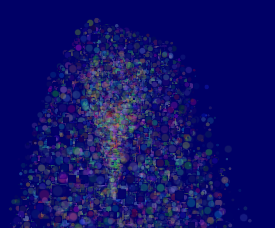
这样ParticleContainer中的粒子就是排好序的了,显示效果已经变正确了:
延伸课题
动画粒子
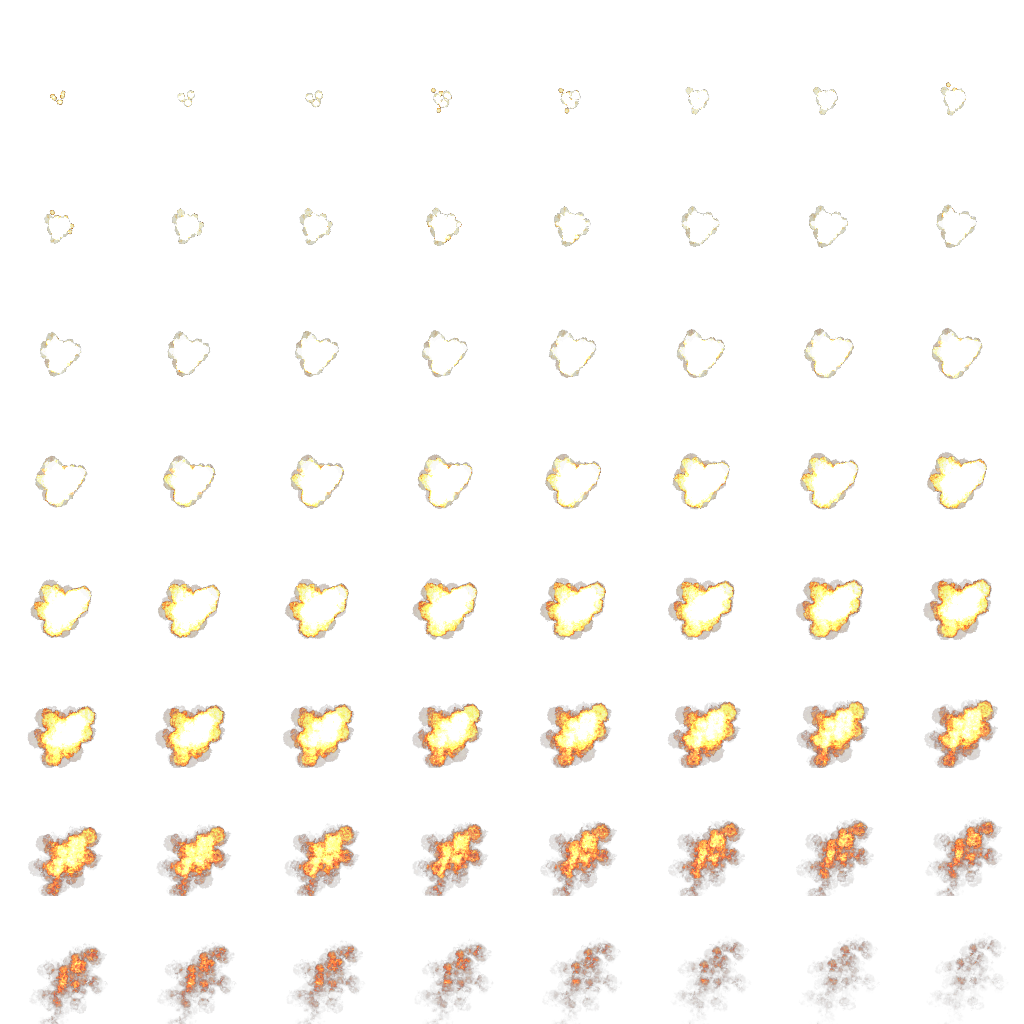
你可以用纹理图集(texture atlas)实现粒子的动画效果。将各粒子的年龄和位置发送到GPU,按照[2D字体一课][2]的方法在shader中计算UV坐标,纹理图集是这样的:
处理多个粒子系统
如果你需要多个粒子系统,有两种方案可选:要么仅用一个粒子容器,要么每个粒子系统一个。
如果选择将所有粒子放在一个容器中,那么就能很好地对粒子进行排序。主要缺陷是所有的粒子都得使用同一个纹理。这个问题可借助纹理图集加以解决。纹理图集是一张包含所有纹理的大纹理,可通过UV坐标访问各纹理,其使用和编辑并不是很方便。
如果为每个粒子系统设置一个粒子容器,那么只能在各容器内部对粒子进行排序。这就导致一个问题:如果两粒子系统相互重叠,我们就会看到瑕疵。不过,如果你的应用中不会出现两粒子系统重叠的情况,那这就不是问题。
当然,你也可以采用一种混合系统:若干个粒子系统,各自配备纹理图集(足够小,易于管理)。
平滑粒子
你很快就能发现一个常见的瑕疵:当粒子和几何体相交时,粒子的边界变得很明显,十分难看:
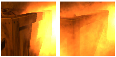
(image from http://www.gamerendering.com/2009/09/16/soft-particles/ )
一个通常采用的解决方法是测试当前绘制的片断的深度值。如果该片断的深度值是“较近”的,就将其淡出。
然而,这就需要对Z-Buffer进行采样。这在“正常”的Z-Buffer中是不可行的。你得将场景渲染到一个[渲染目标][3]。或者,你可以用glBlitFrameBuffer把Z-Buffer内容从一个帧缓冲拷贝到另一个。
http://developer.download.nvidia.com/whitepapers/2007/SDK10/SoftParticles_hi.pdf
提高填充率
当前GPU的一个主要限制因素就是填充率:在16.6ms内可写片段(像素)数量要足够多,以达到60FPS。
这是一个大问题。由于粒子一般需要很高的填充率,同一个片段要重复绘制10多次,每次都是不同的粒子。如果不这么做,最终效果就会出现上述瑕疵。
在所有写入的的片段中,很多都是毫无用处的:比如位于边界上的片段。你的粒子纹理在边界上通常是完全透明的,但粒子的网格却仍然得绘制这些无用的片段,然后用与之前完全相同的值更新颜色缓冲。
这个小工具能够计算纹理的紧凑包围网格(这个也就是用glDrawArraysInstanced()渲染的那个网格):
[http://www.humus.name/index.php?page=Cool&ID=8][4]。Emil Person的网站上也有很多精彩的文章。
粒子物理效果
有些应用中,你可能想让粒子和世界产生一些交互。比如,粒子可以在撞到地面时反弹。
比较简单的做法是为每个粒子做光线投射(raycasting),投射方向为当前位置与未来位置形成的向量。我们将在[拾取教程][5]。但这种做法开销太大了,你没法做到在每一帧中为每个粒子做光线投射。
根据你的具体应用,可以用一系列平面来近似几何体(译注:k-DOP),然后 对这些平面做光线投射。你也可以采用真正的光线投射,将结果缓存起来,然后据此近似计算附近的碰撞(也可以兼用两种方法)。
另一种迥异的技术是将现有的Z-Buffer作为几何体的粗略近似,在此之上进行粒子碰撞。这种方法效果“足够好”,速度快。不过由于无法在CPU端访问Z-Buffer(至少速度不够快),你得完全在GPU上进行仿真。因此,这种方法更加复杂。
如下是一些相关文章:
[http://www.altdevblogaday.com/2012/06/19/hack-day-report/][6]
[http://www.gdcvault.com/search.php#&category=free&firstfocus=&keyword=Chris+Tchou’s%2BHalo%2BReach%2BEffects&conference_id=][7]
GPU仿真
如上所述,你可以完全在GPU上模拟粒子的运动。你还是得在CPU端管理粒子的生命周期——至少在创建粒子时。
可选方案很多,不过都不属于本课程讨论范围。这里仅给出一些指引。
- 采用变换反馈(Transform Feedback)机制。Transform Feedback让你能够将顶点着色器的输出结果存储到GPU端的VBO中。把新位置存储到这个VBO,然后在下一帧以这个VBO为起点,然后再将更新的位置存储到前一个VBO中。
原理相同但无需Transform Feedback的方法:将粒子的位置编码到一张纹理中,然后利用渲染到纹理(Render-To-Texture)更新之。 - 采用通用GPU计算库:CUDA或OpenCL。这些库具有与OpenGL互操作的函数。
- 采用计算着色器Compute Shader。这是最漂亮的解决方案,不过只在较新的GPU上可用。
请注意,为了简化问题,在本课的实现中
ParticleContainer是在GPU buffer都更新之后再排序的。这使得粒子的排序变得不准确了(有一帧的延迟),不过不是太明显。你可以把主循环拆分成仿真、排序两部分,然后再更新,就可以解决这个问题。
